This chapter presented the basic techniques of estimating demand functions and forecasting future sales and prices. Estimation of demand functions is most often accomplished using the technique of regression analysis. Two specifications for demand, linear and log-linear, are presented in this chapter. When demand is specified to be linear in form, the coefficients on each of the explanatory variables measure the rate of change in quantity demanded as that explanatory variable changes, holding all other explanatory variables constant. In linear form, the empirical demand specification is
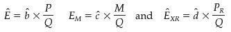
Q = a + bP + cM + dPR
where Q is the quantity demanded, P is the price of the good or service, M is consumer income, and PR is the price of some related good R. The estimated demand elasticities are computed as
(3.0K)
As in any regression analysis, the statistical significance of the parameter estimates can be assessed by performing t-tests or examining p-values.
When demand is specified as log-linear, the demand function is written as
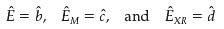
Q = aP b M c P d R
In order to estimate the log-linear demand function, it is converted to natural logarithms:
ln Q = ln a + b ln P + c ln M + d ln PR
In log-linear form, the elasticities of demand are constant, and the estimated elasticities are
(2.0K)
To choose between these two specifications of demand, a researcher should consider whether the sample data to be used for estimating demand are best represented by a demand function with varying elasticities (linear demand) or by one with constant elasticity (log-linear demand). When price and quantity observations are spread over a wide range of values, elasticities are likely to vary, and a linear specification with its varying elasticities is usually a more appropriate specification of demand. Alternatively, if the sample data are clustered over a narrow price (and quantity) range, a constant-elasticity specification of demand, such as a log-linear model, may be a better choice than a linear model.
The method of estimating the parameters of an empirical demand function depends on whether the price of the product is market-determined or manager-determined. Managers of price-taking firms do not set the price of the product they sell; rather, prices are endogenous or "market-determined" by the intersection of demand and supply. Managers of price-setting firms set the price of the product they sell by producing the quantity associated with the chosen price on the downward-sloping demand curve facing the firm. Since price is manager-determined rather than market-determined, price is exogenous for price-setting firms.
When estimating industry demand for price-taking firms, complications arise because of the problem of simultaneity. The simultaneity problem refers to the fact that the observed variation in equilibrium output and price is the result of changes in the determinants of both demand and supply. Because output and price are determined jointly by the forces of supply and demand, two econometric problems arise when a researcher tries to estimate the coefficients of industry demand: the identification problem and the simultaneous equations bias problem.
The identification problem involves determining whether it is possible to trace out the true demand curve from the sample data. Industry demand is identified when supply includes at least one exogenous variable that is not also in the demand equation. The problem of simultaneous equations bias arises when price is an endogenous variable, as it is when price is market-determined for price-taking firms. In order for the standard or ordinary least-squares (OLS) regression procedure to yield unbiased parameter estimates, all explanatory variables must be uncorrelated with the random error term in the demand equation. An endogenous variable is always correlated with the error term in both the demand and supply equations. (This can be verified by examining the reduced form equation for Q, which shows how Q is related to all the exogenous variables and error terms in the system.) Because price is an explanatory variable in the demand equation, and an endogenous variable in the case of price-taking firms, a simultaneous equations bias will result when the OLS procedure is used to estimate demand. The simultaneous equations bias is eliminated by estimating the parameters of the industry demand equation using 2SLS.
When estimating the demand curve facing a price-setting firm—a firm that can control or set the price of its product by varying its own level of production—the problem of simultaneity does not arise. The demand curve for price-setting firms is estimated using the ordinary least-squares (OLS) method of estimation.
Statistical forecasting models can be subdivided into two categories: time-series models and econometric models. Time-series forecasts use the time-ordered sequence of historical observations on a variable to develop a model for predicting future values of that variable. Time-series models specify a mathematical model representing the generating process, then use statistical techniques to fit the historical data to the mathematical model.
The simplest time-series forecast is a linear trend forecast where the generating process is assumed to be the linear model Qt = a + bt. Using time-series data on Q, regression analysis is used to estimate the trend line that best fits the data. If b is greater (less) than 0, sales are increasing (decreasing) over time. If b equals 0, sales are constant over time.
When data exhibit cyclical variation, such as seasonal patterns, dummy variables can be added to the time-series model to account for the seasonality. If there are N seasonal time periods to be accounted for, N − 1 dummy variables are added to the demand equation. Each dummy variable accounts for one of the seasonal time periods. The dummy variable takes a value of 1 for those observations that occur during the season assigned to that dummy variable and a value of 0 otherwise. This type of dummy variable allows the intercept of the demand equation to take on different values for each season—the demand curve can shift up and down from season to season.
In contrast to time-series models, econometric models use an explicit structural model to explain the underlying economic relations. Econometric forecasting can be employed to forecast future industry price and sales or to forecast future demand for price-setting firms. The three steps for forecasting industry price and sales are
We illustrated this process by forecasting future copper price and consumption. The three steps for forecasting the future demand for a price-setting firm are
We illustrated this process by forecasting the future demand facing a pizza restaurant.
When making forecasts, analysts must be careful to recognize that the further into the future the forecast is made, the wider the confidence interval or region of uncertainty. Incorrect specification of the demand equation (as well as supply in the case of simultaneous equations forecasts) can seriously undermine the quality of a forecast. An even greater problem for accurate forecasting is posed by the occurrence of structural changes that cause turning points in the variable being forecast. Forecasts often fail to predict turning points. While there is no satisfactory way to account for unexpected structural changes, forecasters should note that the further into the future you forecast, the more likely it is that a structural change will occur.
This chapter concludes Part II of the text on demand analysis. In Part III of the text, we will present the theory of production and cost. We also will describe the empirical techniques used to estimate production functions and the various cost equations used by managers to make output and investment decisions.
| To learn more about the book this website supports, please visit its Information Center. |
| 2005 Tata McGraw-Hill Any use is subject to the Terms of Use and Privacy Policy. Tata McGraw-Hill is one of the many fine businesses ofThe McGraw-Hill Companies. |